Theia produces atmospheric-corrected surface reflectance images over about 5 million km2 using the MAJA software.
These single-date products (level 2A) are then processed monthly with the WASP software to produce 45-day cloud-free (so-called level 3A) syntheses.
These two products 2A (single date) and 3A (monthly) are available in our download catalog and retain the basic characteristics of Sentinel-2 images, i.e. a geographical coverage of 100x100km and the 13 spectral bands.
On the contrary, the map layers diffused here are the result of an assembly of the 100x100kms products to make a continuous product (called mosaic), diffused in WM(T)S layers and limited to 3 bands for on-screen display.
Three by-products are thus diffused:
A cartographic layer including the three spectral bands red green blue (natural colors),
A map layer in false colors Near Infrared, Red, Green (respectively associated with the colors Red, Green, Blue of the screen),
A black and white map layer showing the NDVI weather index. Pixel value 0 corresponds to NDVI values <=0, with a linear increase to reach a pixel value of 255 for an NDVI=1. The brighter the pixels, the more vegetated the footprint,
An NDVI map layer in false colors ranging from dark brown (no vegetation, low NDVI) to green (high veg index).
The availability Sentinel-2 imagery with its unique characteristics (290 km swath, 10 to 60 m spatial resolution, 5-day revisit cycle with 2 satellites, 13 spectral bands) enables the implementation of land cover map production systems for the delivery of accurate information with the appropriate frequency.
The French Theia Land Data Centre has set up a Land Cover Scientific Expertise Centre in order to implement an fully operational automatic land cover map production system (iota2) using mostly Sentinel-2 image time series. The LULC product is updated once a year and contains ~17 thematic classes mapped at 10 m resolution.
Legend layer Snow
Current state of snow cover for metropolitan France and part of the bordering countries.
This layer presents the daily updated visualization of the snow cover obtained by a temporal synthesis of the acquisitions observed during the last 27 days.
The light blue color of the legend means that snow has been detected via a last acquisition without clouds if this acquisition was made during the last 15 days.
This is not freshly fallen snow, but snow that is guaranteed to be present recently.
The dark blue color indicates that snow was detected during an acquisition observed between 15 and 27 days
before the current date and that all subsequent acquisitions were cloudy.
The white color indicates that all acquisitions during the last 27 days were cloudy
The overlay indicates that snow has never been observed on this pixel in the last 27 days
Note that the atmospheric correction data needed for the calculation are currently available with a 7 day delay.
The most recent acquisitions available for processing are therefore at least 7 days old.
Snow observed on the 15 last days
Snow observed between 15 and 27 days
Clouds
Nodata
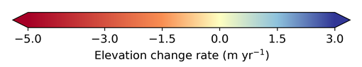
Glacier elevation change rate between 2000 and 2019
Surface elevation change rates of all glaciers and their vicinity (10 km buffer) between 2000 and 2019, from the study of [Hugonnet et al. (2021)](DOI soon) which is the reference to cite when using or plotting these data.
The products can be downloaded by tiles of 1° x1° and by period by accessing the links displayed when passing the cursor on a given tile. Bulk downloading is available at the links at the bottom of this page.
Elevation changes are distributed at a horizontal resolution of 100 m x 100 m and for the 5-year periods of 2000–2004, 2005–2009, 2010–2014 and 2015–2019, the 10-year periods of 2000–2009 and 2010–2019 and the full 20-year period of 2000–2019.
Periods refer to inclusive calendar years of 1st January to 1st of January (e.g., 2000–2004 is January 1, 2000 to January 1, 2005).
Elevation changes are provided as annual rates (in meters per year), allowing comparison of changes between different subperiods. The following colormap is used in all instances :
The glaciers mapped are based on the Randolph Glacier Inventory 6.0.
The surface elevation change estimation derives from fitting Gaussian Process regression to time series of elevation observations from multiple Digital Elevation Models (DEMs).
DEMs are primarily generated and corrected from the Advanced Spaceborne Thermal Emission and Reflection Radiometer (ASTER) stereo imagery [ASTL1A].
Code and guides to manipulate the dataset at different scales are available on a dedicated GitHub repository.
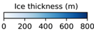
Glaciers Thickness (m)
The product "ice thickness distribution" is derived from the study of Millan et al. (2022).
This is the first comprehensive mapping of ice thicknesses based on glacial flow velocities (cf. product "glacier surface flow velocity"),
for more than 200,000 glaciers on Earth.
This dataset provides a better understanding of the distribution of ice masses on Earth and can be used to initialize models of glacier evolution.
The thicknesses of the glaciers are distributed at a horizontal resolution of 50 m and are representative of the decade 2010-2020. The color scale is in meters
The ice thickness distribution is estimated from the surface flow velocity and the surface slope using the Shallow Ice Approximation (SIA) method.
Slopes were calculated using three different digital elevation model sources, with ASTER GDEM v3 (Abrams et al., 2020), TanDEM-X (DLR, 2018)
and the ArcticDEM from Worldview (Porter et al., 2018). The inversions are calibrated using in situ ice thickness measurements from the
Glacier Thickness Database, when available.
More scientific information is available in Millan et al., 2019, doi: 10.3390/rs11212498
a href="https://doi.org/10.3390/rs11212498">https://doi.org/10.3390/rs11212498 and Millan et al., 2022,
Nature Geoscience https://doi.org/10.1038/s41561-021-00885-z and its supplement.
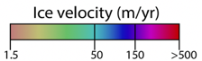
The product "glacier surface flow velocity" for the period 2017-2018 comes from the study of Millan et al. (2022).
This is the first comprehensive mapping of the ice flow velocities for more than 200,000 world's glaciers outside the ice sheets.
This dataset provides a better understanding of the flow dynamics of glaciers, and was used to estimate of the distribution of ice thicknesses (cf. product “ice thickness”).
Glacier flow velocities are distributed at a horizontal resolution of 50 m and represent an average over the period 2017-2018. The color scale is in m/an :
The estimate of glacier surface flow velocities comes from image cross-correlation applied on optical and radar satellite observations, primarily Sentinel-2 (S2), Landsat-8 (L8) and Sentinel-1 (S1).
These sensors make systematic acquisitions with a revisit period ranging from 2 to 16 days.
Surface flow velocities are calculated using all possible image pairs, for time interval ranging from 5 (S2), 6 (S1) ou 16 days (L8), up to more than a year.
The displacement fields obtained for different time interval (defined by the date of acquisition of the images) are averaged over the entire 2017-2018 period in order to ensure exhaustive coverage of the glaciers.
 Snow observed on the 15 last days
 Snow observed between 15 and 27 days
 Clouds
 Nodata
 Theia Cartographic layers : Land Use Land Cover, monthly composites...